
Quartile Calculator
Use our free Quartile Calculator to easily find Q1, Q2 (median), Q3, interquartile range (IQR), minimum, maximum, and dataset range in seconds.


| Quartile Statistics | |
|---|---|
| First Quartile (Q1) | 25 |
| Second Quartile (Q2) | 55 |
| Third Quartile (Q3) | 75 |
| Interquartile Rang (IQR) | 50 |
| Median = Q2 (x˜) | 55 |
| Minimum | 10 |
| Maximum | 100 |
| Range (R) | 90 |
There was an error with your calculation.
Last updated: June 3, 2026
Table of Contents
- Quartiles
- Quartiles Calculation
- Interquartile range
- Minimum and maximum values
- Range of a set
- Quartile Calculations Applications in Real World
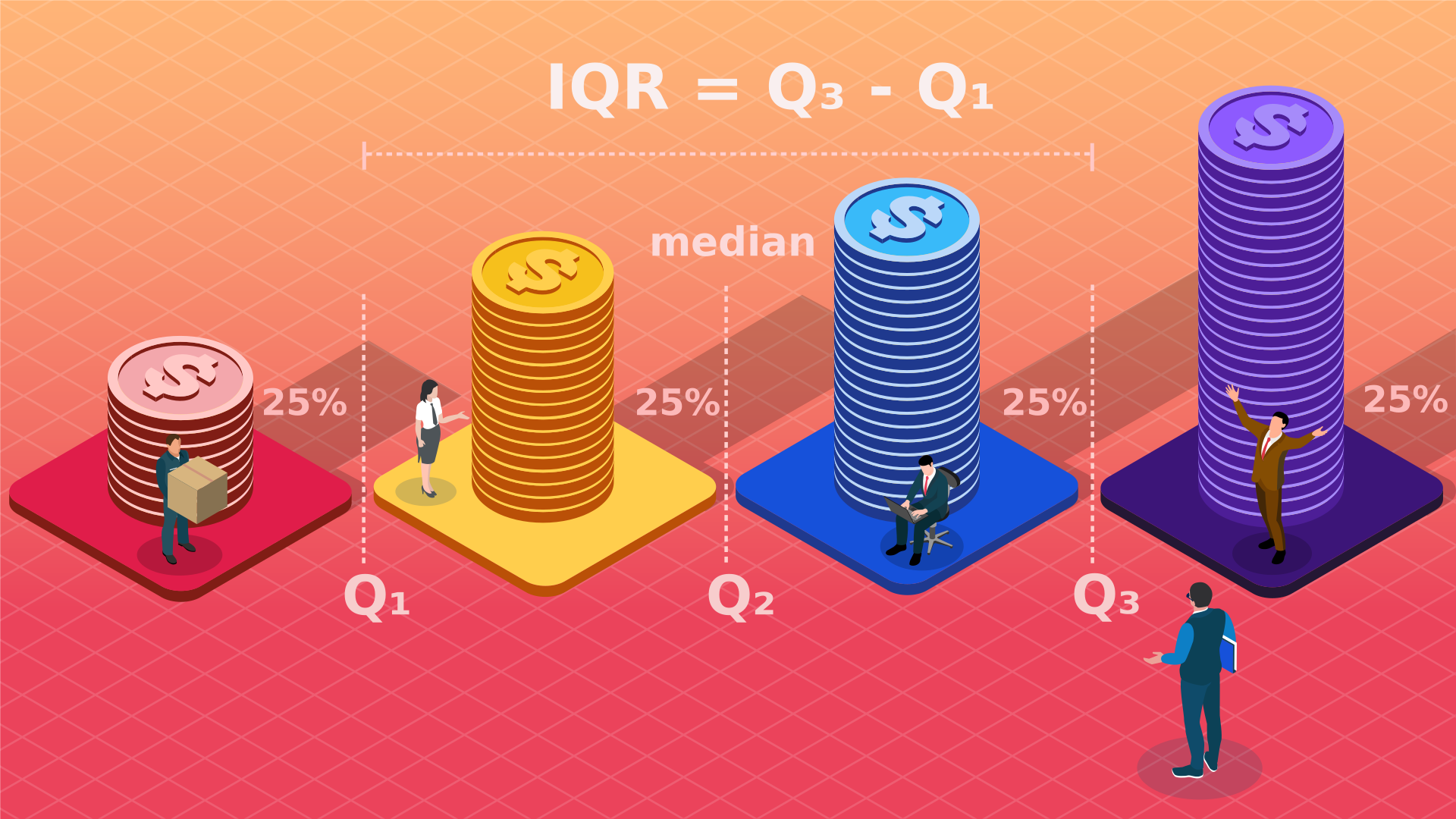
Our online quartile calculator is an essential statistical tool for quickly finding the five-number summary needed for Box-and-Whisker plots. This versatile statistics calculator will instantly determine the first quartile (Q1), second quartile (Q2 or median), third quartile (Q3), minimum value, and maximum value of any given dataset. Additionally, it accurately calculates both the interquartile range (IQR) and the total range.
Simply type or paste your raw data into the input field and click the “Calculate” button. Please ensure you separate each number using a comma or a space.
Quartiles
Quartiles are vital statistical measures of position. They help describe where a specific value stands in relation to the rest of the values in a dataset.
By design, quartiles divide an ordered dataset (arranged in ascending order) into four equal sections, or quarters. Each of these sections contains an equal number of data points. In statistics, we typically calculate three main quartiles for any dataset:
- First quartile (Q1 or the lower quartile)
- Second quartile (Q2 or the median)
- Third quartile (Q3 or the upper quartile)
The first quartile (Q1) is the value that separates the bottom 25% of the ordered data from the top 75%. In other words, 25% of the data points fall strictly below Q1, while 75% sit above it. This is equivalent to the 25th percentile of the dataset.
The second quartile (Q2) is the value that divides the dataset directly in half, separating the bottom 50% from the top 50%. Therefore, 50% of the data lies below Q2, and 50% lies above it. The second quartile is exactly equal to the median, as well as the 50th percentile of the dataset.
The third quartile (Q3) is the value that separates the bottom 75% of the ordered data from the top 25%. This means 75% of the items are lower than Q3, while the remaining 25% are strictly greater. This corresponds to the 75th percentile of the dataset.
Quartiles Calculation
To calculate quartiles manually, you can follow these simple steps:
- Arrange the data in ascending order.
- Find the median of the data values. This is the second quartile.
- Find the median of the data values which are below the second quartile. This is the first quartile.
- Find the median of the data values which are above the second quartile. This is the third quartile.
Example 1
The following dataset represents the starting salaries of newly graduated accountants from a local college. Find the median (Q2), lower quartile (Q1), and upper quartile (Q3) for these starting salaries, and interpret the results.
$55,000, $60,000, $52,000, $45,000, $74,000, $75,000, $48,000, $58,000, $72,000, $66,000, $45,000, $50,000, $54,000, $65,000, $71,000
Solution
First, we will arrange the data in increasing (ascending) order.
$45,000, $45,000, $48,000, $50,000, $52,000, $54,000, $55,000, $58,000, $60,000, $65,000, $66,000, $71,000, $72,000, $74,000, $75,000
Then, we will find the location of the second quartile (the median).
$$Second\ quartile(Q2)=\left(\frac{N+1}{2}\right)^{th}item=\left(\frac{15+1}{2}\right)^{th}item=8^{th}item=58,000$$
Next, find the median of the data values strictly below Q2 to determine Q1.
$45,000, $45,000, $48,000, $50,000, $52,000, $54,000, $55,000
First quartile (Q1) = $50,000
Next, find the median of the data values strictly above Q2 to determine Q3.
$60,000, $65,000, $66,000, $71,000, $72,000, $74,000, $75,000
Third quartile (Q3) = $71,000
You can interpret these quartile results as follows:
25% of the newly graduated accountants earn less than $50,000, while the top 25% earn more than $71,000. Exactly 50% of these graduates earn more than $58,000, and the remaining 50% earn less than that.
As seen in the example above, when working with an odd number of data points, the quartiles correspond to actual original data values. However, with an even number of data points, the quartiles may not map directly to the initial values. Let’s modify the first example to demonstrate this.
Example 2
Assume you missed one salary entry from the data in Example 1. The missing salary is $95,000. Find the revised median (Q2), lower quartile (Q1), and upper quartile (Q3) for the updated starting salaries.
Solution
First, arrange the updated dataset in increasing order.
$45,000, $45,000, $48,000, $50,000, $52,000, $54,000, $55,000, $58,000, $60,000, $65,000, $66,000, $71,000, $72,000, $74,000, $75,000, $95,000
Then, we will find the position of the quartiles.
$$Second\ quartile(Q2)=\left(\frac{N+1}{2}\right)^{th}item=\left(\frac{16+1}{2}\right)^{th}item=8.5^{th}item$$
$$Second\ quartile(Q2)=\frac{8^{th}item+9^{th}item}{2}=\frac{58,000+60,000}{2}=59,000$$
Now, divide the dataset at the median into two distinct groups. Find the median of the data values below Q2 to calculate Q1.
$45,000, $45,000, $48,000, $50,000, $52,000, $54,000, $55,000, $58,000
First quartile (Q1)=($50,000 + $52,000)/2 = $51,000
Next, find the median of the data values above Q2 to calculate Q3.
$60,000, $65,000, $66,000, $71,000, $72,000, $74,000, $75,000, $95,000
Third quartile (Q3) = ($71,000 + $72,000)/2 = $71,500
Interquartile range
The difference between the upper quartile (Q3) and the lower quartile (Q1) is known as the interquartile range (IQR).
- Interquartile range (IQR) = Upper quartile - Lower quartile
- Interquartile range (IQR) = Third quartile - First quartile
- Interquartile range (IQR) = Q3- Q1
The IQR calculation effectively eliminates the lowest 25% and the highest 25% of the values in a data array. In other words, the interquartile range focuses purely on the spread of the middle 50% of your data. Because it ignores values below the lower quartile and above the upper quartile, the interquartile range is highly resistant to extreme values and outliers. This completely eliminates the major drawback associated with standard range calculations.
Example 3
Find the interquartile range for Example 1.
Solution
We previously determined the quartiles for this dataset:
- First quartile (Q1) = $50,000
- Second quartile (Q2) = $58,000
- Third quartile (Q3) = $71,000
Let’s apply the above data to the interquartile formula.
Interquartile range (IQR) = Third quartile (Q3)- First quartile (Q1) = $71,000 - $50,000 = $21,000
Example 4
Find the interquartile range for Example 2.
Solution
We previously determined the quartiles for this dataset:
- First quartile (Q1) = $51,000
- Second quartile (Q2) = $59,000
- Third quartile (Q3) = $71,500
Let’s apply the above data to the interquartile range formula.
Interquartile range (IQR) = Third quartile (Q3) - First quartile (Q1) = $71,500 - $51,000 = $20,500
Minimum and maximum values
The minimum value is simply the lowest observation in a dataset. When data is arranged in increasing order, this is naturally the very first value.
Conversely, the maximum value represents the highest observation in a dataset. In an ordered array, this is always the last value.
Identifying the minimum and maximum values is crucial for understanding the overall spread, or dispersion, of your data. The statistical range—the most fundamental measure of dispersion—is calculated directly from these two extreme points.
Example 5
Find the minimum and maximum values of the dataset containing the starting salaries of newly graduated accountants from Example 1.
Solution
We have already arranged the dataset in ascending order as shown below.
$45,000, $45,000, $48,000, $50,000, $52,000, $54,000, $55,000, $58,000, $60,000, $65,000, $66,000, $71,000, $72,000, $74,000, $75,000
The minimum salary is the first data point in the array. Therefore:
The minimum starting salary of newly graduated accountants = $45,000
The maximum salary is the final data point in the array. Therefore:
The maximum starting salary of newly graduated accountants = $75,000
Example 6
Find the minimum and maximum values of the dataset containing the starting salaries of newly graduated accountants from Example 2.
Solution
We have already arranged the dataset in ascending order as shown below.
$45,000, $45,000, $48,000, $50,000, $52,000, $54,000, $55,000, $58,000, $60,000, $65,000, $66,000, $71,000, $72,000, $74,000, $75,000, $95,000
The minimum salary is the first data point in the array. Therefore:
The minimum starting salary of newly graduated accountants = $45,000
The maximum salary is the final data point in the array. Therefore:
The maximum starting salary of newly graduated accountants = $95,000
Range of a set
In statistics, the range is the most basic measure of data dispersion. It is calculated as the absolute difference between the largest (maximum) and smallest (minimum) values within a dataset.
The range of a set = Maximum value - Minimum value
The range of a set = Largest value - Smallest value
The range represents the total distance or spread between the extremes of a dataset, making it a relatively rough measure of dispersion.
Because it depends entirely on just two extreme data points, the range can be easily distorted and biased if those points are outliers. Since it doesn't account for the central data or overall distribution, statisticians generally do not consider the range to be the most robust measure of statistical dispersion.
Example 7
Find the range of the dataset containing the starting salaries of newly graduated accountants from Example 1.
Solution
Previously, we found the minimum and maximum values of the dataset.
The minimum starting salary of newly graduated accountants = $45,000
The maximum starting salary of newly graduated accountants = $75,000
Now, we will apply the above values to the range formula.
The range of a set = Maximum value - Minimum value = $75,000 - $45,000 = $30,000
Example 8
Find the range of the dataset containing the starting salaries of newly graduated accountants from Example 2.
Solution
Previously, we found the minimum and maximum values of the dataset.
The minimum starting salary of newly graduated accountants = $45,000
The maximum starting salary of newly graduated accountants = $95,000
Now, we will apply the above values to the range formula.
The range of a set = Maximum value - Minimum value = $95,000 - $45,000 = $50,000
Quartile Calculations Applications in Real World
Quartile calculations are incredibly useful when analyzing data distribution while simultaneously filtering out extreme outliers. The list below highlights several real-world fields that rely heavily on quartiles to make informed, data-driven decisions:
Human resources - HR professionals calculate salary quartiles before establishing pay ranges within a company. This statistical approach helps eliminate extremely low figures (like trainee stipends) and unusually high figures (resulting from executive experience or specialized talents) from skewing the standard pay scale.
Finance - Financial analysts and planners use quartiles to evaluate historical spending habits. By understanding how past expenses were distributed across quarters, they can create more accurate plans and avoid the pitfalls of over-budgeting or under-budgeting.
Manufacturing - Quartile analysis provides managers with clear data on standard production capabilities. By isolating the middle 50%, they can evaluate typical performance without distortions caused by anomalies like power outages, worker strikes, or sudden material shortages.
Marketing - When marketers analyze competitor pricing strategies, they use quartiles to establish a standard baseline. This allows them to effectively omit the drastically low prices of inferior products and the highly inflated prices of premium luxury brands from their core market analysis.